A Julia/JuMP model for optimal assignment of teachers to school

We were recently approached by a government to optimally allocate teachers to schools. The state has a few hundred secondary schools and is meant to offer a set of subjects in all these schools. But there are a number of classrooms without a teacher allocated. To close these “gaps”, a new cohort of teachers were trained to join the existing set of teachers. They asked us how these new teachers should be assigned while taking operational and logistical constraints into account. These kinds of problems are notoriously hard to solve optimally¹. Operational Research offers clever techniques to search the solution space for optimal solutions.

In this blogpost, we share how we mathematically defined the optimization problem and solved it using Julia and JuMP. Make sure to also check out this blog post where we discuss lesson learnt when implementing such a model in the socal sector.

What do we want to maximize (or minimize)

We discovered that we might be able to close more of the gap if we could also reassign what classes existing teachers teach at their current school.

There are two ways to frame what the government wishes to do:

1. Minimize the number teachers needed to fill all gaps
2. Maximize the number of classes filled

If we have an excess of teachers, we would clearly want to go with objective 1. Some quick analysis revealed that the gaps were a lot higher than what 1000 teachers could cover. So we converged on objective 2.

In addition, the government wished to prioritize a subset of schools. So our final objective was

Maximize the number of classes filled while giving greater weight to priority schools.

From teachers to teacher types

We discovered that the existing teachers fell into around 40 types. A type is defined by the set of subjects the teacher is qualified to teach. Instead of assigning a particular teacher to a school, we assign a teachers of a given to a school. For example, say Barbara can teach Math and Computer Science. Let’s call this type t1. Instead of assigning Barbara to school A, we assign 1 teacher of type t1 to the school.

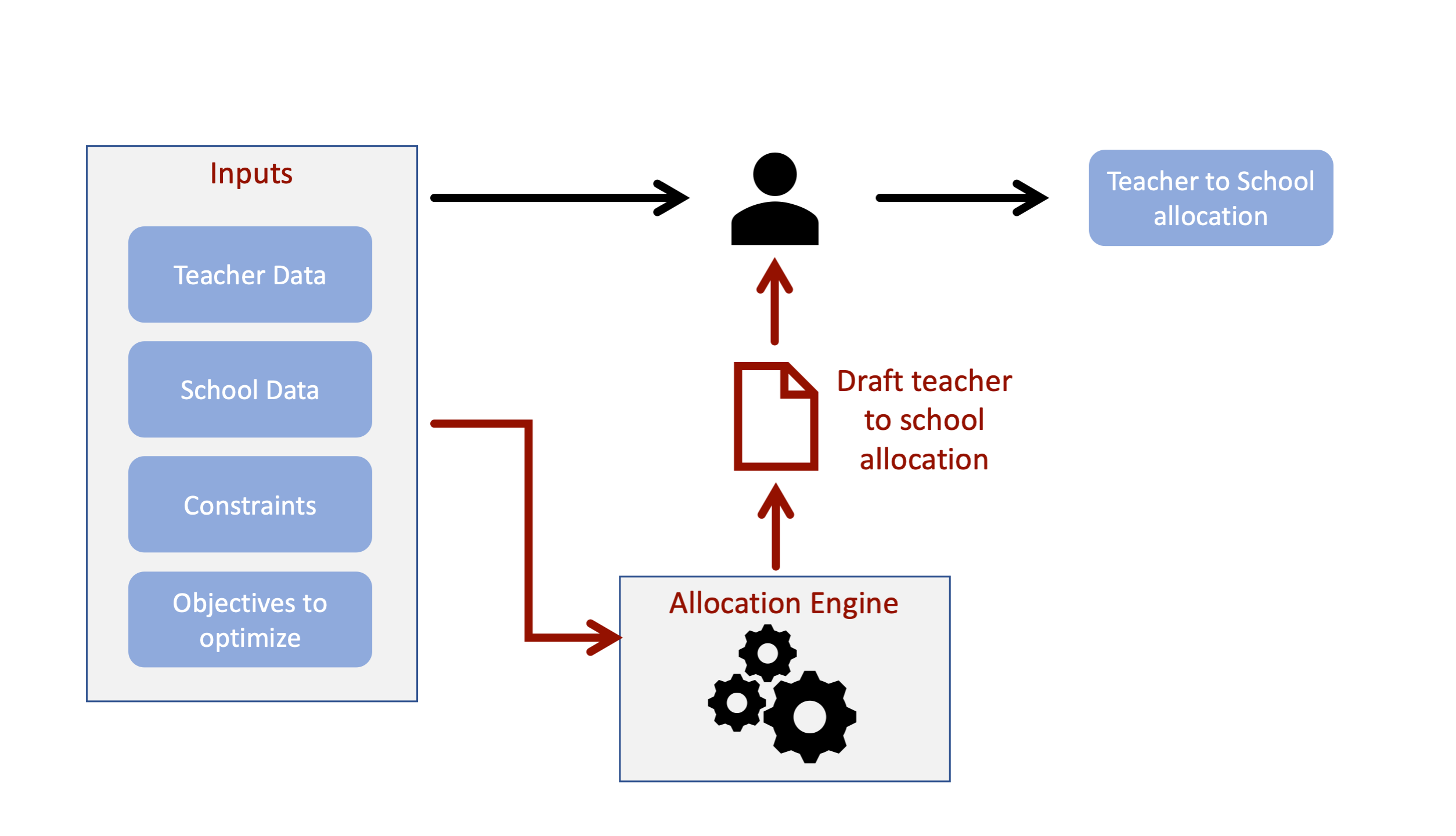
One advantage of this is that it reduces the number of variables since instead of a 3000 variables i.e. one for each existing and new teacher, we now only have around 40 variables². This makes life a lot easier for the solver as it substantially reduces the search space. The second advantage is a bit more subtle. It allows for local knowledge and human discretion to be incorporated in the final teacher allocation. See “Allow for a human in the loop” in this blogpost for more details.

Let’s build the model.

Mathematical model

We represent the allocation of teachers to schools and classes as a matrix $\mathbf{A}$ with integer terms $A_{stb}$ as the number of classes a teacher of type $t$ teaches at school $s$ for subject $b$. We also define a matrix $\mathbf{L}$ with integer terms $L_{st}$ as the number of teachers of type $t$ assigned to school $s$.

What data do we have?

We have access to the following datasets

• $D_{sb}$: The demand for classes of subject $b$ at school $s$
• $E_{st}$: The number of teacher of type $t$ currently at school $s$
• $Q_{tb}$: 1 if teacher type $t$ can teach subject $b$ else -1
• $N_{t}$: The number of new teachers of type $t$
• $U_{s}$: 1 if the schools $s$ is should be prioritized, 0 otherwise

Let’s also define some of sets we have:

• $\mathbf{S}$ is the set of all schools
• $\mathbf{B}$ is the set of all subjects
• $\mathbf{T}$ is the set of all teacher types

The objective function

We want to maximize the total number of classes taught (by a teacher) at schools.

$$ \begin{equation*} \text{maximize},,, {\sum_{stb} A_{stb}} + \lambda \left(\sum_{tb} A_{stb}\right) \cdot U_{s} \end{equation*} $$

Where $\lambda$ is a positive integer that roughly equates to the relative importance of a class at a priority school versus a non-priority school. Setting $\lambda$ to 0 would mean that classes at priority schools are not prioritized over other schools.

Constraints

Having defined the objective function, we move to defining the constraints using the matrices define above

Constraint 1: You can only teach a positive number or classes.

$$ A_{stb} >= 0\hspace{1em} \forall s \in \mathbf{S}, t \in \mathbf{T}, b \in \mathbf{B} $$

Constraint 2: You cannot allocate more than the given number of teachers of each type

Total teachers of each type available are the new teachers plus the existing teachers for each type. This results in $|\mathbf{T}|$ constraints.

$$ \sum_{s} L_{st} <= N_{t} + \sum_{s} E_{st} \hspace{1em} \forall t \in \mathbf{T} $$

Constraint 3: Existing teacher stay at their current school

At a minimum, the final allocation must have the same number of teachers or each types as it has currently. This results in $|\mathbf{S}| \times |\mathbf{T}|$ constraints.

$$ L_{st} >= E_{st} \hspace{1em}\forall s \in \mathbf{S}, t \in \mathbf{T} $$

Constraint 4: Don’t allocate more than the demand at a school

At each school, the maximum number of classes staffed is less than or equal to the demand at that school. This creates $|\mathbf{S}| \times |\mathbf{B}|$ constraints.

$$ \sum_{t} A_{stb} <= D_{sb} \hspace{1em}\forall s \in \mathbf{S}, b \in \mathbf{B} $$

Constraint 5: Teacher can only teach classes for which they are qualified

We are taking a Hadamard product of each slice of $\mathbf{A}$ across the $s$ dimension. So this creates $|\mathbf{S}| \times |\mathbf{B}| \times |\mathbf{T}|$ constraints.

$$ A_{s’tb} \circ Q_{tb} >= 0 \hspace{1em}\forall s’ \in S $$

Constraint 6: Teacher can teach a maximum of 5 classes

Similar to the previous constraint, we are taking slices of $\mathbf{A}$ across the $s$ dimension. This creates $|\mathbf{S}| \times |\mathbf{B}| \times |\mathbf{T}|$ constraints.

$$ \sum_{b} A_{stb} <= 5 L_{st}\hspace{1em}\forall s,t $$

Note: This also sufficient to define $L_{st}$. You don’t need an implication constraint explicity linking $\mathbf{A}$ with $\mathbf{L}$

Writing up the model in Julia + JuMP

Julia is a very concise and readable language and JuMP is very intuitive and pretty decent documentation. This post is not meant to go into the nuts and bolts of Julia or JuMP so we don’t elaborate on the code. We provide the sample code below to shows how the objective function and constraints can be coded.³

using JuMP
using HiGHS
using CSV
using DataFrames


# ------ Data Setup -------
# -------------------------

N_CLASSES_PER_TEACHER = 5
LAMBDA = 5

school_need_df = DataFrame(CSV.File("data/needs_school_x_subject.csv"))
existing_teachers_df = DataFrame(CSV.File("data/existing_school_x_tt.csv"))
teacher_capability_df = DataFrame(CSV.File("data/qualification_tt_x_subject.csv"))
new_teachers_df = DataFrame(CSV.File("data/available_tt.csv"))
priority_df = DataFrame(CSV.File("data/priority_dummy.csv"))

## As matrices
school_need = school_need_df[:, 2:end] |> Matrix
existing_tt = existing_teachers_df[:, 2:end] |> Matrix
teacher_capability = teacher_capability_df[:, 2:end] |> Matrix
teacher_capability[teacher_capability .== 0] .= -1
new_teachers = new_teachers_df.Numberofteachers
priority_schools = priority_df.priority

n_types = size(teacher_capability)[1]
n_schools, n_subjects = size(school_need)

# ------ Define Model -------
# ---------------------------

model = Model(HiGHS.Optimizer)
set_optimizer_attribute(model, "presolve", "on")
set_optimizer_attribute(model, "time_limit", 1500.0)

@variable(model, A[1:n_schools, 1:n_types, 1:n_subjects] >= 0, Int)
@variable(model, types_used[1:n_schools, 1:n_types], Int)

@constraint(model, positive_assignment, A .>= 0)

@constraint(model,
            keep_existing_teachers[s in 1:n_schools, t in 1:n_types],
            types_used[s, t] >= existing_tt[s, t])

@constraint(model,
            total_teacher_limits[t in 1:n_types],
            sum(types_used[:, t]) <= (new_teachers[t] + sum(existing_tt[:, t])))

@constraint(model,
            capacity_of_teachers[s in 1:n_schools, t in 1:n_types],
            sum(A[s, t, :]) .<= N_CLASSES_PER_TEACHER * types_used[s, t])

@constraint(model,
            max_gap_covered[s in 1:n_schools, b in 1:n_subjects],
            sum(A[s, :, b]) <= school_need[s, b])

@constraint(model,
            capability_match[s in 1:n_schools],
            A[s, :, :] .* teacher_capability[:, :] .>= 0)


@objective(model,  Max, sum(A) + LAMBDA * sum(sum(A, dims=[2, 3]) .* priority_schools) )

optimize!(model)

Final words

In this technical post we discuss how we defined an optimization problem in math and then in code. But as every good data scientist knows, the actual modelling is only 10% of the work. The remaining 90% was spent working closely with the stakeholder to define the problem, collating datasets, and (of course) cleaning and manipulating them into the matrices needed for the model.

If you are interested in some of the softer and, in some ways, more challenging aspects of the project, check out this other blogpost on the same project.