Clustering algorithms for grid-based sampling

TL;DR: In this blog post, we will describe a custom clustering algorithm we designed to efficiently cluster grids into enumeration areas for grid-based sampling

The DSEM team at IDinsight is the technical workhorse for project teams, and nearly every piece of technical work we do involves grouping things by some measure of similarity. Let me explain.

For our work with Educate Girls (EG), we predicted the number of out-of-school girls (OOSGs) in villages across northern India. The information that EG really needed, however, was which villages they should visit to implement their programs to get girls back into school. So, in addition to predicting OOSGs, we needed to group villages that were geographical neighbours (i.e. within a 25km radius of each other), and also had high numbers of OOSGs. In another project, we are helping a project team in Morocco cluster rooftops to create enumeration areas for a survey. Similarly, our automated enumerator-target assignment tool SurveySparrow, which allows survey teams to efficiently assign enumerators to targets based on distance, also groups targets into clusters that can easily be visited by an enumerator. For our automated grid-based sampling tool, we constructed a custom clustering algorithm to combine grids into clusters based on survey-specific criteria.

A non-authoritative crash course on clustering analysis¹

Clustering analysis refers to a class of methods that allows us to group data points in a dataset into clusters, such that all the points within a cluster are similar to each other on some metric, and points in different clusters are dissimilar. Think the Sorting Hat for Hogwarts houses.

Mathematically speaking, given a set of features $X$, we want to find patterns within the features $X$ by grouping them. Clustering analysis can in principle be applied to any kind of feature $X$, as long as we can mathematically express some notion of similarity between two data points $X_i$ and $X_j$. The feature $X$ can also be arbitrarily high-dimensional, although computational complexity of clustering algorithms scales with the dimensionality of $X$.

Clustering for grid-based sampling

In grid-based sampling, we use population density maps to construct enumeration areas for surveys (for a detailed explanation, see this blog post). The density maps consist of grids (of a specific resolution e.g. 30m x 30m or 100m x 100m). We need to cluster these grids into enumeration areas that enumerators must traverse while visiting targets for the survey.

Thus for clustering, the features $X$ are the coordinates (latitude and longitude) of a grid, and we define “similarity” as the great-circle distance (GCD) between two grid coordinates. However, we cannot obtain enumeration areas simply by clustering nearby grids together: we typically want to satisfy other constraints on the clusters as well. For example, each cluster must have certain minimum number of targets, cannot exceed a maximum number of targets, and must conform to a specific geographic size. Note that these are constraints we want to impose, in addition to our similarity metric i.e. GCD.

This is a hard problem since we cannot use common clustering algorithms out-of-the-box to solve it. With k-means clustering, we need to know the number of clusters we want to create a priori, and we cannot naturally impose the additional constraints we described above. In order to get usable clusters for survey teams, we need to do hyperparameter sweep to determine the best number of clusters and re-run k-means with different initializations until all constraints are satisfied – more on this approach in a follow-up blog post!

More sophisticated density- or distribution-based clustering methods (e.g. DBSCAN) could allow us more control than k-means, without having to use sweeps and multiple initialisations for the algorithm. However, these methods entail estimating or postulating a probability distribution for the collection of points in a cluster – this could again be time-consuming and resource-intensive. More importantly, they are likely to fail when the dataset size is small, and can be unnecessarily complex and hard to interpret: it is difficult to describe or estimate a distribution over coordinates for grids.

Given these considerations, we developed our own greedy algorithm. This algorithm specifically deals with the population and cluster radius constraints that are required for grid-based sampling.

A custom algorithm for clustering grids

The custom algorithm (pseudo-code at the bottom of this post) works on a dataset consisting of grids, coordinates for each grid and the corresponding metric $m$ by which we want to constrain the cluster size e.g. population, number of rooftops in the grid, etc.

With this algorithm, we need to specify 3 parameters before we can begin grouping clusters:

1. the maximum allowed distance $d$ between 2 points in a cluster (this indirectly controls the geographic area of a cluster)
2. the lower bound $m_l$ for the metric by which we want to constrain cluster size
3. the upper bound $m_u$ for the metric constraining cluster size.

We start by computing the distance between each grid and all the other grids in our dataset i.e. $GCD(X_i, X_j) \forall i, j$ where $i, j$ denote grids in the dataset. We then group “nearby” grids falling within the specified distance in (1) together, while ensuring that the sum of the metric for all grids within a cluster falls within the range specified in (2) and (3). It works in 2 steps:

• Step 1: For a particular grid (say, grid $i$), we loop through all the other grids in our dataset, and add them to a list if they fall within the specified distance of grid $i$ i.e. $GCD(X_i, X_j) \leq d$ (note that a grid A also belongs to this list). We only keep adding grids to this list until the sum of the metric $m$ for all the grids in the list falls in the specified range i.e. $m_l \leq \sum_j m_j \leq m_u, \forall j \in$ list of grids . We continue this process for each grid in the dataset, while ensuring that no grid gets assigned to 2 lists. After one pass through the dataset, the resulting lists make our first set of clusters. Note, not all the grids in the dataset will get assigned a cluster when we do this i.e. we could have isolated grids.
• Step 2: We loop through this initial group of clusters and unassigned points, and combine them with other nearby clusters while satisfying the specified distance and metric criteria, until as many clusters as possible fall within the specified metric range $[m_l, m_u]$. This can still leave unassigned points, in particular when the distance and metric criteria are in conflict e.g. we cannot add more grids to a cluster even if they lie within $d$, because the cluster will exceed the specified metric range; or conversely, we cannot add more grids to the cluster to bring the cluster metric into the specified range, because no more grids lie within the specified distance $d$.

However, we can exert some control over this by defining a fourth criterion: which of $m_l$ and $m_u$ is the stricter bound. This results in two variants:

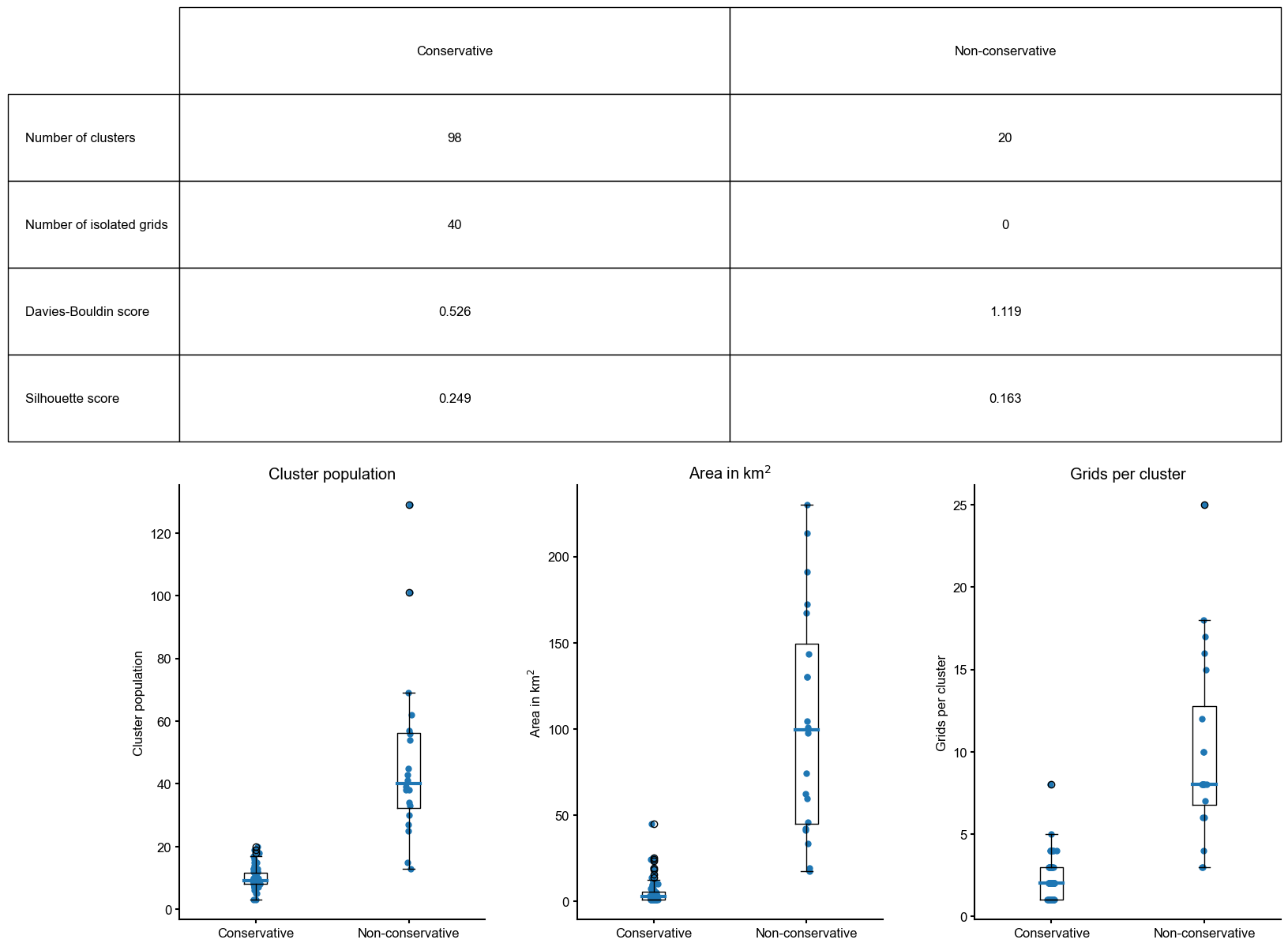
1. conservative, where $m_l$ is strict: in both step 1 and 2, the algorithm stops adding grids to clusters as soon as the cluster metric has satisfied the specified lower bound i.e. $\sum_j m_j \geq m_l$. This variant leads to more clusters and more isolated isolated points overall. Each cluster formed using this variant typically contains fewer points, is spatially smaller and better separated from other clusters.
2. non-conservative, where $m_u$ is strict: in both step 1 and 2, the algorithm keeps adding points to clusters until the cluster metric has satisfied the specified upper bound i.e. $\sum_j m_j \leq m_u$. This variant leads to fewer clusters and fewer isolated points overall. Each cluster formed using this variant typically contains more points, is spatially larger and not well-separated from other clusters.

The advantages of this algorithm are:

• Its enormous flexibility – it is agnostic to the metric we use to constrain the clusters.
• We are guaranteed to get roughly similar-sized clusters spatially and with respect to the metric (when the upper and lower bounds are not widely different).
• It gives us fine-grained control on the clustering.

On the downside,

• We cannot specify the number of clusters, and we may end up with unassigned or isolated points.
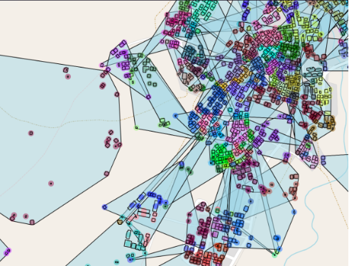
• It also leads to overlapping clusters when the grids are densly packed. This means we can’t just give the boundaries of the clusters to surveyors and say “visit every house inside this boundary”. Instead suveyors also have to pay attention to which specific house / grid belongs to the cluster they are surveying, and take care only to visit those, and not other houses / grids that lie inside the boundary of a cluster, but don’t belong to the cluster. This makes it very difficult to use these clusters on-the-ground during surveys.
• Finally, these clusters are not confined by geographical features (roads, rivers, mountains, etc.). Once again, this makes it difficult to use the clusters on the ground, since a single cluster could stretch across a highway that an enumerator cannot cross.

What’s next?

We originally developed the algorithm specifically for creating enumeration areas from gridded population density maps. We found that the algorithm is just as effective for clustering based on rooftop data, geographic area or any gridded information. We could also update the algorithm to incorporate constraints based on multiple metrics, and combine it with other common clustering algorithms such as k-means depending on the survey requirements. We could also experiment quickly with different values for $d$, $m_l$ and $m_u$, and also with different metrics $m$ for survey planning.

However, the algorithm produces clusters that are very difficult to operationalize: the overlapping issue in particular, is difficult to fix without manually re-drawing boundaries or imposing additional constraints that lead to sub-optimal results. The algorithm also does not account for geographical barriers (mountains, rivers, highways) while creating clusters, and assumes that the gridded information is accurate, which may not always be true. We have since found that tweaking k-means clustering is a much more effective approach for dealing with the overlaps and producing more usable clusters (look out for a blog post on this soon!)

We are currently piloting both the greedy and the updated k-means algorithm on multiple survey projects and gathering feedback on what is useful and feasible for survey teams to work with. We are hoping to make continuous improvements to our clustering approaches for different surveys, even as we engage in more data collection work (via DataDelta).

Algorithm pseudocode:

#---------------------------------------------------------------------------
# Step 1: Form initial clusters
#---------------------------------------------------------------------------
Inputs: dataframe, minimum_pop, maximum_pop, grid_distance_matrix, radius, sufficiency_condition
# sufficiency_condition = minimum_pop OR maximum_pop
Outputs: dataframe_with_initial_clusters

for i, row in randomly_sort(dataframe):
  if row[population] < sufficiency_condition and row[cluster] is None:
	nearest_grids <- nearest unassigned grids by grid_distance_matrix,
                 	inside radius, and population < maximum_pop
	cluster <- subset of nearest grids + row, such that minimum_pop <= total population <= maximum_pop

	if cluster is empty:
  	cluster <- row
  else:
	cluster <- row

  dataframe_with_initial_clusters[i] = cluster
#---------------------------------------------------------------------------


#---------------------------------------------------------------------------
# Step 2: Re-assign under-allocated clusters
#---------------------------------------------------------------------------
Inputs: dataframe_with_initial_clusters, minimum_pop, maximum_pop, grid_distance_matrix, radius, sufficiency_condition
# sufficiency_condition = minimum_pop OR maximum_pop
Outputs: dataframe_with_final_clusters

for i, row in randomly_sort(dataframe_with_initial_clusters):
  if row_combine_population < sufficiency_condition:
	nearest_clusters <- nearest clusters by grid_distance_matrix, within radius,
                    	with combined_population < maximum_pop
	new_cluster <- row + subset of nearest_clusters such that minimum_pop <= total population <= maximum_pop

  else:
	new_cluster <- row

  dataframe_with_final_clusters[i] = new_cluster