Data quality check for hierarchical linear data with outliers


In this post, I discuss how IDinsight’s DSEM team implemented a data quality check for pairs of variables displaying linear relationships. We explain why we chose a Bayesian model, and the tweaks we made to address the hierarchy and outliers in data. We will also see how to implement the model using PyMC3.
Last year, IDinsight built a tool for a national government agency to automatically check the quality of the data reported by dozens of district governments every month. Some of these checks were simple, like checking for null values, illegal values, and outliers.
Another check we implemented was what we call “ratio checks”1. We observed that many of the variables consistently displayed linear relationships in pairs. There were logical reasons for these relationships, too, for example when the two variables represent counts of related events. We wanted to check that new values would also follow these patterns.
 For a pair of variables with a linear relationship, we want to check that a new point (x, y) follow the same pattern.
We had three requirements for this check.
Requirement 1. The results should be intuitive. Something like a probability that a new point is anomalous given past data would be useful.
Requirement 2. These linear relationships look slightly different for different districts. We want an efficient model that takes into account both similarities and differences across the districts.
Requirement 3. Past data itself contains outliers. There might have been data entry errors or a rare event in certain districts that resulted in one variable taking an extreme value relative to the other variable. We want the model to be robust to occasional outliers.
Below, we discuss how robust hierarchical Bayesian linear regression addressed these concerns, and show how to implement it using PyMC3.
Quantify uncertainty using a Bayesian model
Requirement 1. The results should be intuitive.
For a pair of variables $x, y$ with a linear relationship, we want to estimate $ p(y|x) $ based on past data. We can flag a point $(x_i, y_i)$ as an outlier if it’s unlikely that we observe a value as extreme as $y_i$.
We could fit a simple linear regression model:
$$ y = \alpha + \beta x + \epsilon \\ \epsilon \sim \text{Normal}\left(0, \sigma^2\right) $$
which can be viewed as
$$Y|x\sim \text{Normal}\left(\alpha + \beta x, \sigma^2\right).$$
In Bayesian statistics, we want to find the distribution of the model parameters $\theta = {\alpha, \beta, \sigma}$ given the data that we already observed. This is called the posterior, written $p(\theta|y)$2.
Once we have the posterior, we can evaluate how likely it is to see some new data $y’$ (given $x’$) by integrating $p(y’|\theta)$ over the posterior. This distribution, $p(y’|y)$, is called the posterior predictive distribution.
To get the posterior, we first set prior distributions over the parameters as follows:
$$ \begin{align*} \alpha&\sim \text{Normal}(0, 5)\\ \beta&\sim \text{Normal}(0, 2)\\ \sigma&\sim \text{HalfNormal}(5) \end{align*} $$
This represents our initial belief about what values of the parameters are likely.
import pymc3 as pm

with pm.Model() as basic_linear_model:
    # 1. Priors
    alpha = pm.Normal("α", 0, sigma=5)
    beta = pm.Normal("β", mu=0, sigma=2)
    sigma = pm.HalfNormal("σ", sigma=5)

    # 2. Likelihood
    mu = alpha + beta * x
    likelihood = pm.Normal("y", mu=mu, sigma=sigma, observed=y)

# Visualize
pm.model_to_graphviz(basic_linear_model)

Now, we simulate the posterior using MCMC sampling, which is simple with PyMC3:
with basic_linear_model:
    # 3. Inference
    trace = pm.sample(1000, return_inferencedata=True)
The trace contains samples from the posterior distribution, and its histogram gives us an approximation of the posterior.
| Definitions | |
|---|---|
| Posterior distribution ($p(\theta|y)$) | Distribution over model parameters given the observed data |
| Posterior predictive distribution ($p(y’|y)$) | Distribution over unobserved data based on the observed data and the posterior distribution |
| Credible interval | Interval into which an unobserved parameter falls with a given probability. |
| Highest density interval (HDI) | The narrowest credible interval for a given probability. |
Making predictions
Now that we have the posterior $p(\theta|y)$ we can approximate the posterior predictive distribution $p(y’|y)$ for new data $y’$: We first sample parameters from the posterior, $\theta’\sim p(\theta|y)$, and then sample from $p(y’|\theta’)$.
To sample from the posterior predictive in PyMC3, we have to modify the code slightly. We need to tell the model that $x$ is training data (see 0. Data) that can be replaced with some test data later on(see 4. Test data).
with pm.Model() as basic_linear_model:
    # 0. Data
    x_data = pm.Data("x_data", x_train_scaled)

    # 1. Priors
    alpha = pm.Normal("α", 0, sigma=5)
    beta = pm.Normal("β", mu=0, sigma=2)
    sigma = pm.HalfNormal("σ", sigma=5)

    # 2. Likelihood
    mu = alpha + beta * x_data
    likelihood = pm.Normal("y", mu=mu, sigma=sigma, observed=y)

    # 3. Inference
    trace = pm.sample(1000, return_inferencedata=True)

    # 4. Test data
    pm.set_data({"x_data": x_test_scaled})

    # 5. Posterior predictive distribution
    ppc = pm.sample_posterior_predictive(trace, var_names=["y"])
ppc["y"] contains samples drawn from the posterior predictive distribution. Using this we can compute credible intervals at various probabilities. For example, for a given $x’$, there is 95% probability that the corresponding $y’$ falls within the 95% credible interval $(y_a, y_b)$, i.e. $p(y_a< y’<y_b|x’) = 95%$.3 If $y’$ falls outside this range, we would flag the data point as anomalous.4
 95% highest density credible interval (HDI) of the posterior predictive distribution $p(y’|y)$ (in orange area) compared to original data
A hierarchical model for hierarchical data
Requirement 2. We want an efficient model that takes into account both similarities and differences across the districts.
In our data, the same pair of variables had slightly different intercepts and variances across different districts. A single linear model fit across the entire dataset would ignore this heterogeneity. On the other hand, if we fit a different linear model for each district, we’d lose out on the shared patterns across the districts and might end up with noisy estimates.
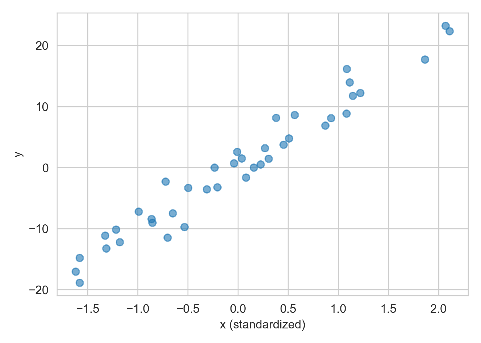
 Toy hierarchical data. Each group displays a linear pattern, but with differing slopes and variances.
Rather than a single global model or dozens of individual models, we chose a hierarchical (also known as partial pooling or multilevel) model, where we assume that the parameters of $p_i(y|x)$ for each group (in our case, district) come from a common distribution.
In the first level, we set hyperpriors for the global means ($\mu_\alpha, \mu_\beta$) and variances ($\sigma_\alpha, \sigma_\beta$) of group-wise intercepts ($\alpha_i$’s) and group-wise slopes ($\beta_i$’s).
$$ \begin{align*} \mu_\alpha&\sim \text{Normal}(0, 2)\\ \sigma_\alpha&\sim \text{HalfNormal}(5)\\ \mu_\beta&\sim \text{Normal}(1, 2)\\ \sigma_\beta&\sim \text{HalfNormal}(5) \end{align*} $$
In the next level, the parameters above are plugged into the group-wise priors. This is where we take the group-wise variations into account. For each group $i$, the priors are
$$ \begin{align*} \alpha_i&\sim \text{Normal}(\mu_\alpha, \sigma_\alpha^2)\\ \beta_i&\sim \text{Normal}(\mu_\beta, \sigma_\beta^2) \end{align*} $$
Then our likelihood for each observation $j$ in group $i$ is
$$Y_{ij}|x_{ij}\sim \text{Normal}(\alpha_i+\beta_i x_{ij}, \sigma^2)$$
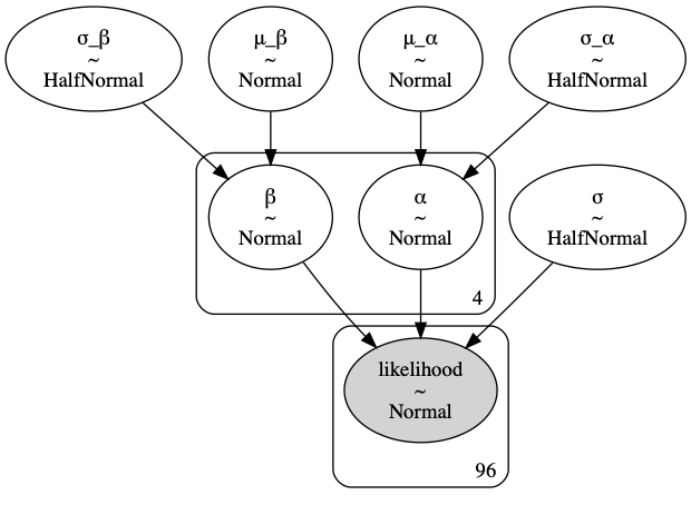
A hierarchical model
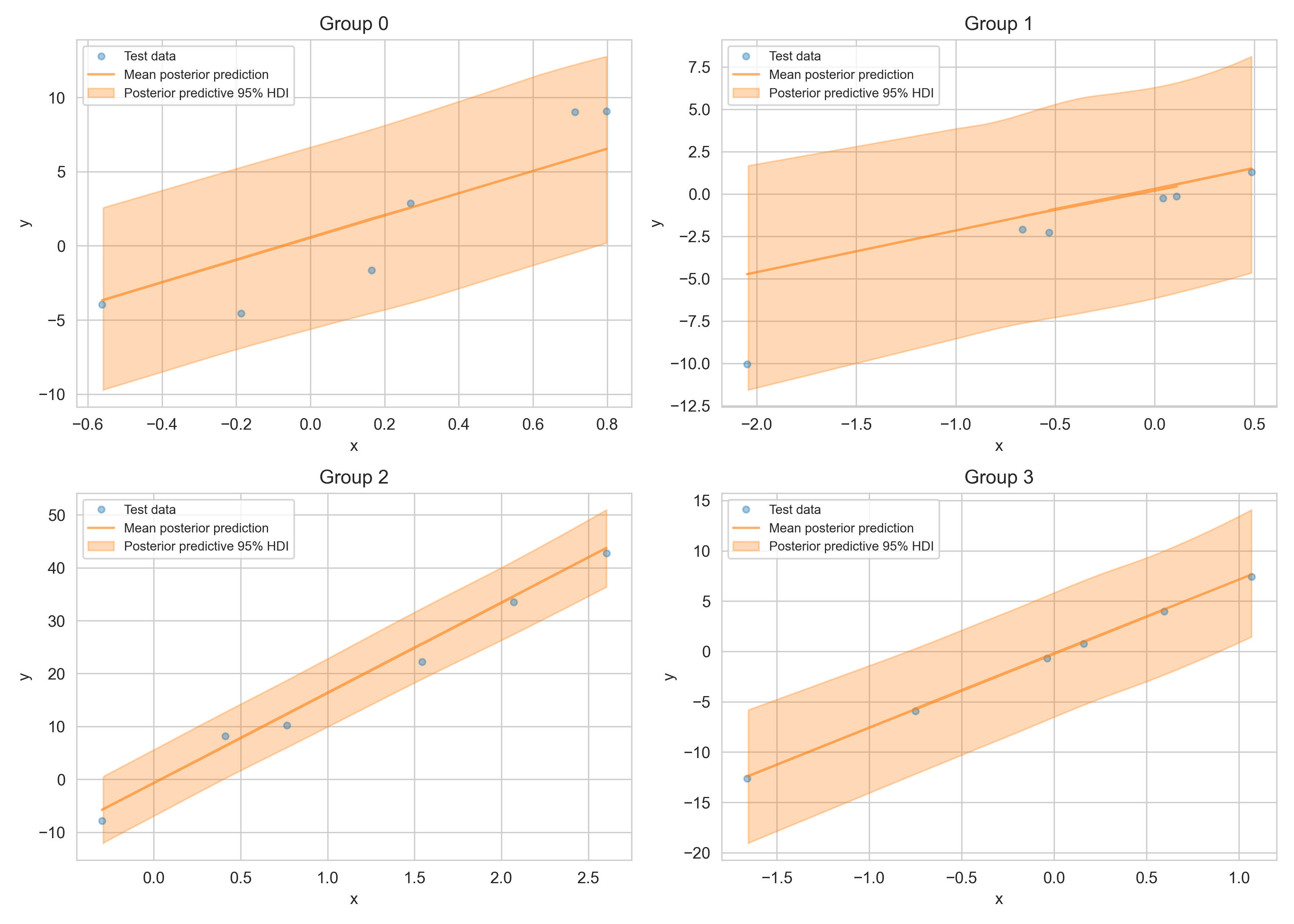 95% HDI of the posterior predictive distribution (orange area) of test data (blue markers).
Robust regression for data with outliers
Requirement 3. We want the model to be robust to occasional outliers.
Another issue was that the data contained outliers, either due to data entry errors or some rare events. We wanted a model that could robustly handle those points.
 Linear, but with a few outliers
We achieved this by changing the likelihood distribution from Gaussian to Student’s T:
$$Y_i|x_i \sim \text{StudentT}(\alpha_i + \beta_i x, \sigma, \nu)$$
Student’s T distribution looks a lot like Gaussian but is more heavy-tailed.5 This means that a few outliers are more likely, and hence will not skew the parameters so much.
Combining this with the hierarchical structure, our code looked like the following. Note the priors for each level of the hierarchy, and that we use shape=n_groups to create district-wise parameters. We also set priors over the parameters for Student’s T distribution.
with pm.Model() as hierarchical_model:
    # 0. Data
    x_data = pm.Data("x_data", x_train_scaled)
    group_index = pm.Data("group_idx", group_ids_train)

    # 1. Priors
    # Level 1
    # Parameters for global intercept
    mu_alpha = pm.Normal("μ_α", mu=0, sigma=2)
    sigma_alpha = pm.HalfNormal("σ_α", sigma=5)
    # Parameters for global slope
    mu_beta = pm.Normal("μ_β", mu=1, sigma=2)
    sigma_beta = pm.HalfNormal("σ_β", sigma=5)

    # Level 2
    # We follow https://twiecki.io/blog/2017/02/08/bayesian-hierchical-non-centered/
    # and use uncentered parametrization.
    # Parameters for group-wise intercepts
    a_offset = pm.Normal("α_offset", mu=0, sigma=1, shape=n_groups)
    alpha = pm.Deterministic("α", mu_alpha + a_offset * sigma_alpha)
    # Parameters for group-wise slopes
    b_offset = pm.Normal("β_offset", mu=0, sigma=1, shape=n_groups)
    beta = pm.Deterministic("β", mu_beta + b_offset * sigma_beta)

    # Parameters for likelihood
    nu = pm.Poisson("nu", mu=1, testval=1)
    sigma = pm.HalfNormal("σ", 2)

    # 2. Likelihood
    y_pred = alpha[group_index] + beta[group_index] * x_data
    likelihood = pm.StudentT("likelihood", mu=y_pred, sigma=sigma, nu=nu, observed=y)

    # 3. Inference
    trace = pm.sample(1000, return_inferencedata=True)

    # 4. Test data
    pm.set_data({"x_data": x_test_scaled})

    # 5. Posterior predictive distribution
    ppc = pm.sample_posterior_predictive(trace, var_names=["likelihood"])
Deployment
The existing data quality checks were running on Airflow, with a single data quality check running as a single pipeline. Since inference requires lots of sampling time, we decided to create a separate inference (or “model fitting”) pipeline just for ratio checks. This way, if an error occurs or if the sampling doesn’t converge, we can address the issue without blocking the check, which can be run using the latest stable model.
We defined a regressor class with fit and predict methods. In the model fitting pipeline, the fit method is called on existing data, and a fitted model containing the trace is uploaded to an S3 bucket. In the data quality check pipeline, for the variable pairs $(x, y)$ that require ratio checks, the appropriate model is pulled from S3 and the predict method is called to estimate the posterior predictive distribution for $y$. We check if the actual values of $y$ fall within the HDI of chosen width.
import os


class RobustHierarchicalLinear:
    def __init__(n_chains):
        self.n_chains = n_chains  # number of chains to sample
        self.trace = None

    def fit(x, y, group_index):
        with self.build_model(x, group_index):
            self.trace = pm.sample(
                draws=2000,
                tune=2000,
                chains=self.n_chains,
                cores=os.cpu_count(),
                return_inferencedata=True
            )

    def predict(x, y, group_index, hdi_prob=0.95):
        with self.build_model(x, group_index):
            pm.set_data({"x_data": x, "group_idx": group_index})
            ppc_pred = pm.sample_posterior_predictive(
                self.trace, var_names=["likelihood"]
            )

        likelihood = ppc_pred["likelihood"].reshape(-1, self.n_chains, len(x))
        hdi = az.hdi({"likelihood": likelihood}, hdi_prob=hdi_prob).likelihood
        # Each row in `hdi` now contains the 95% highest density credible intervals for each value of `x`
        # Check if the values in `y` lie inside the intervals:
        check_success = (y >= hdi[:, 0]) & (y <= hdi[:, 1])

        return check_success

    def build_model(x, group_index):
        """Builds and returns a robust hierarchical linear pymc3 model"""
These pipelines can then run on different schedules as required.
 Airflow pipelines of 1) model fitting and 2) prediction as part of data quality checks.
Final thoughts
We created a data quality check called “ratio check” for linearly related variables. In this check, data points that are unlikely given the historical linear relationship would be marked as outliers. To quantify that unlikeliness, we fit a Bayesian model. Since the linear relationships were distinct yet related across different groups, we adopted a hierarchical structure. To handle outliers in the past data, we used Student’s T likelihood instead of the usual Gaussian likelihood. Finally, we wrapped this process in a class with a scikit-learn style API with fit and predict methods and deployed it through two Airflow pipelines: one pipeline calls fit to regularly train an up-to-date model, and another pipeline calls predict when the data quality check is triggered.
Challenges
In this process, we ran into a few difficulties, one of them being the sampling time. To get a more accurate picture of the posterior, we needed to sample thousands of times for each parameter. We also had to try a different hierarchical parametrization for the sampling to converge. It also turned out that using a discrete prior, such as Poisson, for the degrees of freedom in Student’s T distribution was sufficient, rather than using a continuous prior like HalfCauchy, which led to much slower convergence.
Another tricky part was deploying PyMC3 on Airflow, likely because of the way PyMC3 uses theano on the backend. We learned the hard way that the model needs to be rebuilt each time before sampling, and that the only thing that should be saved is the trace. Because we run multiple ratio check pipelines in parallel inside the same docker container, we had to make sure that the theano cache was reset before each sampling.
Future Improvements
Of course, our choice of the model only works if the pairs of variables consistently display linear relationships, across all groups. We picked the pairs for ratio checks based on not just empirical linear relationships but based on whether it is logical or reasonable for them to be linearly related. However, some external shock could change this relationship, as it seemed to have happened in a few of the districts. In one case, one variable continued to increase while the other one lagged behind, changing the slope of the relationship. In another, one of the variables displayed a step change, changing the intercept of the linear model. We will need a more flexible model for these cases.
Currently, we run model diagnostics manually (such as looking at trace plots, effective sample sizes, number of divergences, and $\hat{R}$ values), but these should be integrated into the model fitting pipeline. If any of the diagnostics indicate potential divergence, we can trigger a notification for further human inspection.
Resources
There are a number of details and interesting detours we didn’t mention, but here are some resources for you to dig deeper:
- Prior and Posterior Predictive Checks: a PyMC3 tutorial for checking that our priors give a reasonable predictive distribution, before we look at the data (prior predictive check), and checking if the posterior predictive distribution is reasonable (posterior predictive check).
- GLM: Robust Regression using Custom Likelihood for Outlier Classification: a PyMC3 tutorial on outlier detection. While the robust regression was sufficient for our case, the Hogg method which uses a mixture of a linear model for inliers and another model for outliers.
- Hierarchical Partial Pooling: a PyMC3 tutorial for hierarchical models.
- Why hierarchical models are awesome, tricky, and Bayesian: Thomas Wiecki writes about why one parametrization of hierarchical model might work better than another.
- For a comprehensive reference on Bayesian modelling, see Bayesian Data Analysis by Andrew Gelman, John Carlin, Hal Stern, David Dunson, Aki Vehtari, and Donald Rubin.
This is a misnomer, since we’re checking for the linear relationship and not the ratio of the variables, but we have yet to come up with an appropriate name! ↩︎
Technically, the posterior is conditioned on the observed $x$ and posterior predictive distribution is conditioned on both observed $x$ and new $x’$ values, but we omit them for brevity. ↩︎
An N% credible interval can be found over many different ranges of $y$. We choose the highest density interval (HDI), which captures the same probability over the smallest range of $y$. ↩︎
This intuitive interpretation is in contrast to confidence intervals in frequentist settings. There, a 95% confidence interval only guarantees that the procedure to compute this interval will capture the correct parameter 95% of the time, but we can’t say anything about realized values. ↩︎
In fact, as the degrees of freedom approaches infinity the Student’s T distribution approaches $\text{Normal}(0, 1)$. ↩︎