Bayesian Pattern Recognition for Real World Applications

📚 View all posts in the Graph-based Healthcare Series

Graph-based Healthcare Series — 5

This is the fifth post in an ongoing series on graph-based healthcare tools. Stay tuned for upcoming entries on clinical modeling, decision support systems, and graph-powered AI assistants.

In our previous post, we explored how large language models (LLMs) can simulate realistic pediatric patient encounters based on the IMNCI guidelines. These synthetic notes were grounded in real clinical logic, labeled with structured IMNCI classifications, and validated using a multi-agent verification strategy inspired by the Bayesian Truth Serum (BTS). The result: a high-fidelity dataset of richly annotated, clinically plausible pediatric cases.

In this post, we put that dataset to work—prototyping a Bayesian diagnostic engine that quantifies clinical evidence, scores conditions, and updates probabilities in a way that mirrors how clinicians think.

---

The Big Picture

"How informative is a clinical feature in predicting a diagnosis?"

This question is central to our Bayesian reasoning engine. By grounding the answer in real (or realistically simulated) data, we take a step toward diagnostic systems that are probabilistic, interpretable, and aligned with clinical intuition.

To investigate this, we need detailed patient-level data that captures real-world clinical uncertainty—ambiguity, co-morbidity, and noisy observations. However, as discussed in our previous post, such data is notoriously scarce due to privacy constraints and documentation variability.

So, we turn to the next best thing: synthetic patient cases—generated using clinical logic and rigorously annotated under the IMNCI framework.

But the goal isn’t just to simulate notes. It’s to explore how structured clinical observations can be used to reason under uncertainty—combining partial evidence and updating beliefs in a principled, explainable way.

That’s where Bayesian pattern recognition comes in.

---

Roadmap to Diagnostic Reasoning Using Bayesian Pattern Recognition

Before diving into the technical details, let’s zoom out and look at the big picture.

At a high level, our goal is to understand how individual clinical features—like "blood in stool" or "respiratory rate ≥ 60 bpm"—influence the likelihood of medical classifications such as DYSENTERY or PNEUMONIA. This mirrors how clinicians reason from signs and symptoms toward a diagnosis.

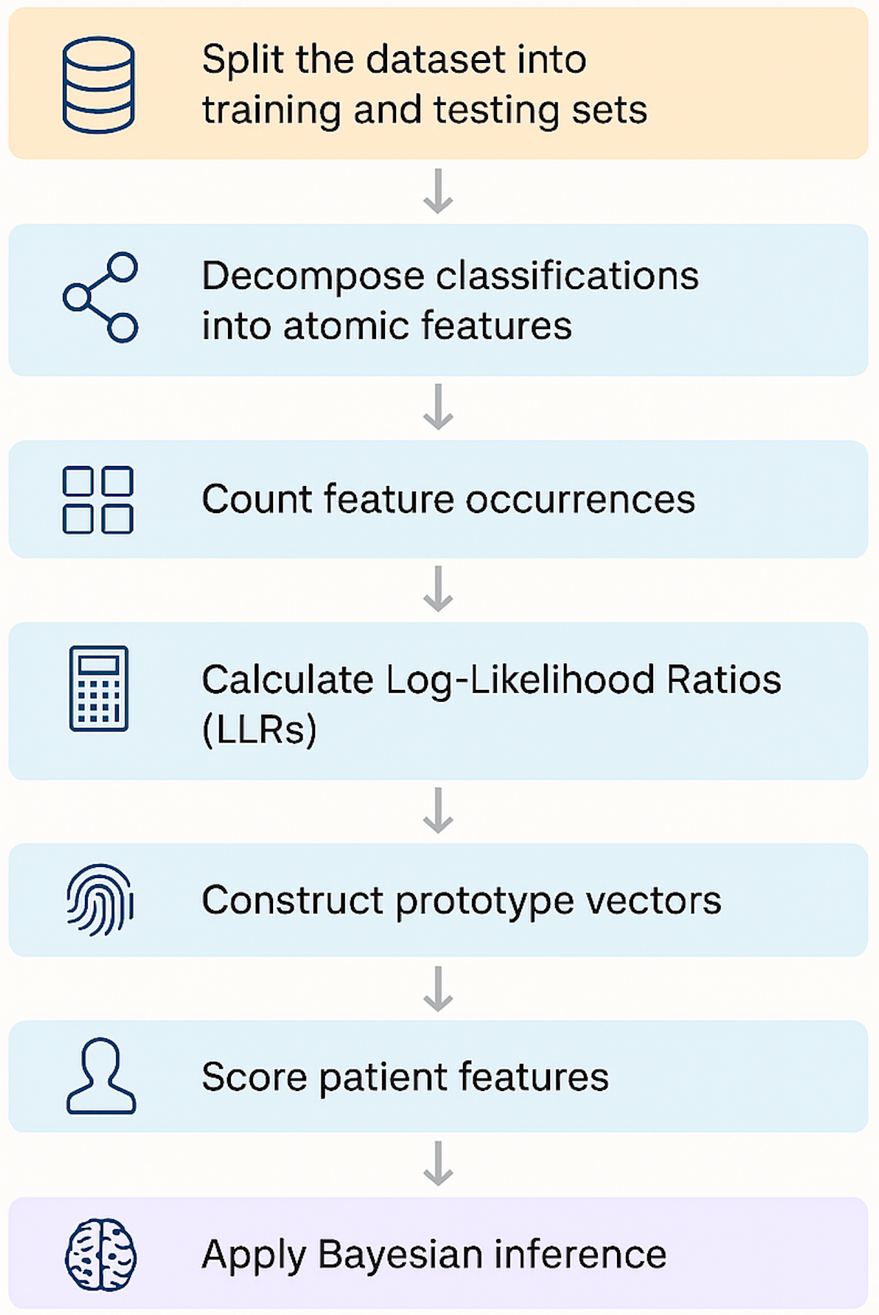
Here’s the step-by-step roadmap:

1. Split the dataset into training and testing sets

   We begin by dividing our synthetic dataset into stratified subsets. Each sample contains ground-truth classifications and the observations supporting them.

2. Decomposing classifications into atomic features

   Classifications are tied to higher-level observations, which we decompose into fine-grained atomic features (e.g., “Yellow skin,” “Infant age < 24 hours”).

3. Count feature occurrences

   We track how often each atomic feature appears when a classification is present or absent. These counts become the statistical foundation for the subsequent steps.

4. Calculate Log-Likelihood Ratios (LLRs)

   For each feature–classification pair, we compute an LLR—a measure of how strongly that feature supports (or contradicts) the diagnosis.

5. Construct prototype vectors

   Using LLRs, we build a diagnostic “fingerprint” for each classification: a vector representing the weighted importance of each feature.

6. Score patient features

   A patient’s feature vector is scored against each prototype using a dot product. The result is an evidence score for every possible classification.

7. Apply Bayesian inference

   Finally, we convert these scores into posterior probabilities using Bayes’ rule—allowing us to reason under uncertainty and account for co-morbid conditions.

The outcome is a lightweight, interpretable diagnostic engine that mirrors the way clinicians synthesize information—ranking possible diagnoses based on evidence and prior knowledge.

---

Splitting the Dataset: Training vs. Testing

The first step in our diagnostic pipeline is dividing the dataset into training and testing sets—a deceptively simple task that requires care when working with multi-label clinical data.

Each patient case in our synthetic dataset includes:

• One or more ground-truth classifications
• A corresponding set of ground-truth observations

For example:

{
  "Baby brought in, very poor feeding according to mother, \"he just won't latch anymore\"... breathing seems rapid, maybe 60 breaths/min... also noticed yellow palms and soles, quite marked. Temp feels cool, checked axilla - 35.3C.": {
    "ground_truth_classifications": [
      "VERY SEVERE DISEASE",
      "SEVERE JAUNDICE"
    ],
    "ground_truth_observations": [
      "Not feeding well",
      "Fast breathing (\u226560 bpm)",
      "Low body temperature (< 35.5\u00b0C) (SEE FOOTNOTE A)",
      "Palms and/or soles yellow"
    ],
    ...
  }
}

Since many cases include multiple classifications (e.g., both SEVERE JAUNDICE and VERY SEVERE DISEASE), we need a splitting strategy that preserves the full label landscape, even for rare conditions.

Stratification is Key

A naive random split can easily exclude rare classifications from the test set entirely and make it impossible to evaluate their performance. To avoid this, we use Multilabel Stratified Shuffle Split, a method from the iterstrat library.

This approach ensures:

• Both training and test sets maintain the same label distribution
• Even rare labels appear in both sets
• The split is random but reproducible, via a fixed random_state

How It Works

• Convert the classification labels into a binary matrix, where each row represents a patient case and each column a classification.

• The stratified split algorithm:

  1. Sorts labels by rarity
  2. Assigns cases to training/test sets while preserving label proportions
  3. Repeats until balanced coverage is achieved

This method is especially important in pediatrics, where co-morbidities are common:

"Infant with yellow eyes and poor feeding"
→ Classifications: JAUNDICE + FEEDING PROBLEM

Without stratification, a random split might push all JAUNDICE cases into the training set and leave the test set blind to it.

Visualizing the Split

Each bar represents a classification. Multilabel stratification ensures both splits retain similar frequencies, even for rare conditions.

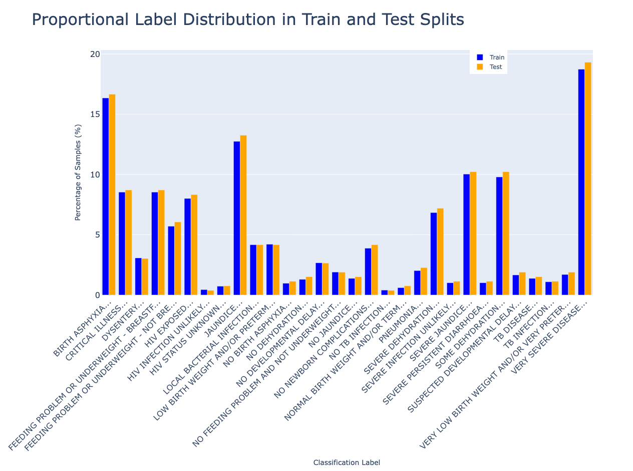
We use a 90/10 train/test split. This gives us enough training data for robust statistics, while holding out a representative test set to evaluate how well our engine generalizes.

In the next section, we’ll explore how high-level IMNCI classifications are mapped to atomic diagnostic features that form the building blocks of probabilistic reasoning.

---

Decomposing Classifications into Atomic Features

Before we can reason probabilistically about clinical diagnoses, we need to define our basic unit of evidence: the atomic feature.

In the IMNCI framework, each classification (e.g., JAUNDICE, DYSENTERY) is linked to one or more structured observations; e.g., clinical statements like:

• "Thrush (ulcers or white patches in mouth)"
• "Skin and eyes yellow and baby is < 24 hrs old"

These observations are rich but coarse-grained. Many encode multiple sub-findings in a single sentence, which limits their usefulness for fine-grained statistical reasoning.

Why Atomic Features?

Take this observation:

"Skin and eyes yellow and baby is < 24 hrs old"

This actually encodes three distinct clinical signs:

• Yellow skin
• Yellow eyes
• Infant age < 24 hours

If we treat the full sentence as one unit, we lose the ability to:

• Attribute diagnostic weight to individual elements
• Capture signal when only part of the observation is present
• Support partial matches (e.g., a baby with yellow eyes but no age data)

By breaking complex observations into atomic features, we enable the model to reason more precisely and flexibly.

Mapping Observations to Features

To perform this decomposition, we prompted an LLM to generate a one-to-many mapping between IMNCI observations and their atomic components. For example:

{
  "Thrush (ulcers or white patches in mouth)": [
    "Oral ulcers",
    "White patches in mouth"
  ],
  "Mother or young infant HIV antibody negative": [
    "Mother HIV antibody: negative",
    "Young infant HIV antibody: negative"
  ],
  "Skin and eyes yellow and baby is < 24 hrs old": [
    "Yellow skin",
    "Yellow eyes",
    "Infant age: < 24 hours"
  ],
  ...
}

This mapping is used to transform each patient case into a flat list of atomic features, which serve as the core inputs for:

• Counting feature–classification associations
• Computing log-likelihood ratios
• Building diagnostic prototypes
• Performing Bayesian updates

What This Allows Us To Do

Atomic features allow the model to:

• Capture diagnostic signal even when only partial observations are present
• Quantify the independent influence of individual signs
• Support explainability (e.g., “Diagnosis X is likely because of features A, B, and C”)

In short, atomic features form the granular evidence layer that powers all subsequent reasoning in our system.

In the next section, we’ll see how counting these features across training data lets us measure how informative each one is.

---

Counting What Matters: Features and Labels

To quantify how informative each clinical feature is, we first need to count how often it appears, both with and without each classification. These counts form the statistical foundation for computing likelihoods and updating diagnostic beliefs.

Why Feature Counts Matter

If “Yellow palms” shows up in most SEVERE JAUNDICE cases but rarely elsewhere, it’s likely a strong diagnostic indicator. But if it's common across many classifications, its signal is diluted.

By capturing feature–label frequencies, we set the stage for computing log-likelihood ratios in the next step.

Step 1: Count Classification Frequencies

We start by tallying how often each classification appears in the training data. These counts reflect condition prevalence and will be used to compute prior probabilities later.

{
  "SEVERE JAUNDICE": 132,
  "FEEDING PROBLEM": 256,
  ...
}

Step 2: Count Features by Classification

Next, we analyze how often each atomic feature co-occurs with each classification.

For every training case:

1. We retrieve its ground-truth classifications
2. For each classification, we collect its associated observations
3. We then convert those observations into atomic features
4. If a feature is present in the note, we increment the count for that feature–classification pair

Importantly, we only increment counts for features that were actually observed in the case. This avoids inflated signals from unrelated features.

Example output:

{
  "Yellow palms": {
    "SEVERE JAUNDICE": 92,
    "MILD JAUNDICE": 12,
    "FEEDING PROBLEM": 0
  },
  "Temperature: < 35.5°C": {
    "VERY SEVERE DISEASE": 67,
    "SEVERE JAUNDICE": 38
  }
}

From Raw Counts to Diagnostic Insight

These tallies provide the raw data for computing log-likelihood ratios, which quantify how strongly each feature supports or contradicts a classification.

They also reveal patterns of diagnostic ambiguity:

• Features common across many conditions may be uninformative
• Features tightly linked to one classification may be high-value signals

In the next section, we’ll transform these raw counts into interpretable evidence scores using log-likelihood ratios.

---

Measuring Evidence: Log-Likelihood Ratios

Now that we’ve counted how often each atomic feature appears with and without each classification, it’s time to measure how informative those features really are.

We do this using Log-Likelihood Ratios (LLRs), a statistical tool that quantifies how strongly a feature supports (or contradicts) a diagnosis.

What is an LLR?

For a given feature \(f\) and classification \(c\), the LLR is defined as:

\[ \text{LLR}_{f,c} = \log \left( \frac{P(f \mid c)}{P(f \mid \neg c)} \right) \]

Where:

• \(P(f \mid c)\): Probability of observing feature \(f\) when classification \(c\) is present
• \(P(f \mid \neg c)\): Probability of observing feature \(f\) when classification \(c\) is absent

To avoid divide-by-zero issues, we apply Jeffreys prior smoothing with a constant \(\alpha = 0.5\):

\[ P(f \mid c) = \frac{k_{\text{pos}} + \alpha}{N_c + 2\alpha}, \quad P(f \mid \neg c) = \frac{k_{\text{neg}} + \alpha}{N_{\neg c} + 2\alpha} \]

Example: High LLR Contrast

Suppose:

• “Yellow palms” appears in 92 cases labeled as SEVERE JAUNDICE
• It also appears in 10 cases not labeled as SEVERE JAUNDICE
• There are 132 total SEVERE JAUNDICE cases in the dataset
• There are 4868 non-SEVERE JAUNDICE cases
• We use a smoothing factor \( \alpha = 0.5 \)

First, calculate the smoothed probabilities:

\[ P(f \mid c) = \frac{92 + 0.5}{132 + 2 \cdot 0.5} = \frac{92.5}{133} \approx 0.695 \]

\[ P(f \mid \neg c) = \frac{10 + 0.5}{4868 + 2 \cdot 0.5} = \frac{10.5}{4869} \approx 0.00216 \]

Then, compute the log-likelihood ratio:

\[ \text{LLR}_{f,c} = \log \left( \frac{0.695}{0.00216} \right) \approx \log(321.76) \approx 5.77 \]

A log-likelihood ratio of 5.77 indicates that the presence of “Yellow palms” makes SEVERE JAUNDICE over 300 times more likely than if the feature were absent—signaling strong diagnostic evidence.

Example: Low/Negative LLR Contrast

Conversely, a feature that appears at similar rates in both positive and negative cases will yield an LLR near zero, indicating low informativeness.

Consider a different feature like “Crying”, which might be common across many cases, regardless of diagnosis.

Suppose:

• “Crying” appears in 45 cases labeled as SEVERE JAUNDICE
• It also appears in 1200 cases not labeled as SEVERE JAUNDICE
• Total SEVERE JAUNDICE cases = 132
• Total non-SEVERE JAUNDICE cases = 4868
• Smoothing factor \( \alpha = 0.5 \)

Compute the smoothed probabilities:

\[ P(f \mid c) = \frac{45 + 0.5}{132 + 2 \cdot 0.5} = \frac{45.5}{133} \approx 0.342 \]

\[ P(f \mid \neg c) = \frac{1200 + 0.5}{4868 + 2 \cdot 0.5} = \frac{1200.5}{4869} \approx 0.247 \]

Now compute the log-likelihood ratio:

\[ \text{LLR}_{f,c} = \log \left( \frac{0.342}{0.247} \right) \approx \log(1.384) \approx 0.325 \]

An LLR of 0.33 is marginal, which indicates that “Crying” is only slightly more associated with SEVERE JAUNDICE than with other conditions.

But suppose instead we had:

• 45 cases with the classification
• 1800 cases without the classification

Then:

\[ P(f \mid \neg c) = \frac{1800 + 0.5}{4868 + 2 \cdot 0.5} = \frac{1800.5}{4869} \approx 0.370 \]

\[ \text{LLR}_{f,c} = \log \left( \frac{0.342}{0.370} \right) \approx \log(0.924) \approx -0.079 \]

Now the LLR is negative, suggesting that “Crying” may actually be less indicative of SEVERE JAUNDICE than of other conditions.

How to Interpret LLR Values

LLR Value	Interpretation
> 1.0	Strong positive evidence
~0.0	Neutral or uninformative
< 0.0	Weakly contradictory or widely distributed

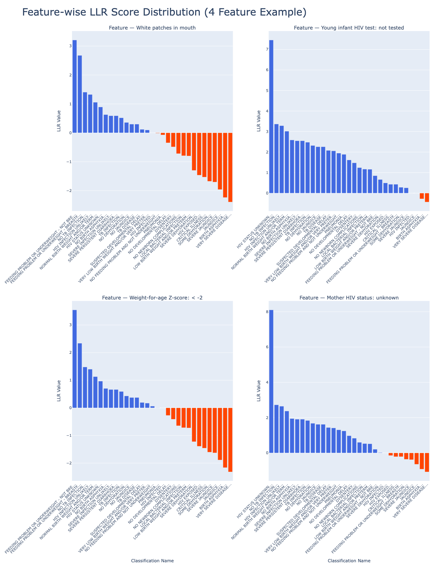
Visualizing LLR Distributions

To get a sense of the overall landscape, we can visualize the distribution of LLR scores across example features and classifications:

Some features (right-skewed bars) are highly discriminative for specific diagnoses, while others cluster around zero and offer little signal.

From Statistics to Structure

Log-likelihood ratios quantify association and also give us a principled way to transform raw feature counts into diagnostic evidence scores.

These scores act as the statistical backbone of our system, enabling it to:

• Capture the relative diagnostic strength of each atomic feature
• Build prototype vectors that summarize what each classification “looks like”
• Support probabilistic reasoning over complex, co-morbid patient presentations

In the next section, we’ll use these LLRs to construct diagnostic fingerprints: weighted feature profiles that let us compare new patients against known disease patterns.

---

Building Diagnostic Fingerprints From LLRs

Once we’ve computed log-likelihood ratios for each feature–classification pair, the next step is to aggregate those scores into prototype vectors—diagnostic fingerprints that represent each medical classification in a structured, interpretable way.

Each prototype vector represents a single medical classification (like SEVERE JAUNDICE or PNEUMONIA) as a weighted map of features, where the weights are derived from our previously computed LLRs.

What’s a Prototype Vector?

A prototype vector represents a single medical condition (e.g., SEVERE JAUNDICE) as a mapping of features to their LLR weights:

{
  "SEVERE JAUNDICE": {
    "Yellow palms": 8.74,
    "Yellow eyes": 1.16,
    "Temperature: Normal": -2.34,
    ...
  }
}

Each feature's weight reflects how strongly it supports or contradicts the condition.

Using LLRs as Weights

LLRs quantify how discriminative each feature is for a specific condition. By directly using these values as weights, our prototype vectors reflect presence and informative strength:

• A feature with high LLR appears often with the classification but rarely without
• Features common across many classifications are downweighted naturally

This means we’re not just capturing whether a feature appears but also how much it should influence the final decision.

Optional: Normalizing the Scores

In practice, we typically use raw LLRs to retain the full magnitude of evidence strength, especially when scoring patients via dot products. However, in downstream applications (e.g., neural architectures or ensemble models) the following normalized forms can provide bounded inputs and smoother training behavior. We support:

Method	Range	Use Case
tanh(LLR)	-1 to +1	Capped but retains sign and scale
sigmoid(LLR)	0 to 1	Smooth probabilities
Scaled sigmoid	-1 to +1	Bounded + centered on zero

Prototype Vectors vs. Text Embeddings

It’s tempting to equate prototype vectors with text embeddings of IMNCI classification descriptions. However, they operate in different spaces:

Vector Type	Represents	Behavior
Text embeddings	Language semantics (phrases, syntax, wording)	Clusters by similar language
Prototype vectors	Evidence profiles (atomic clinical features)	Separates by diagnostic patterns

In short:

• Text embeddings live in a language space: they tell you which diagnoses are semantically similar.
• Prototype vectors live in a clinical-evidence space: they tell you which diagnoses share the same underlying patterns of symptoms and signs.

They’re different by design and not meant to overlap or be interchangeable.

Visualizing the Difference Between Text Embeddings and Prototype Vectors

We can also visualize these differences by projecting both embedding spaces into two dimensions using UMAP.

Text Embedding Space

Text embeddings cluster closely based on linguistic similarity. Labels like "20: SEVERE JAUNDICE", "21: JAUNDICE", and "22: NO JAUNDICE" occupy nearby positions because their language is similar (even if their diagnostic roles are very different).

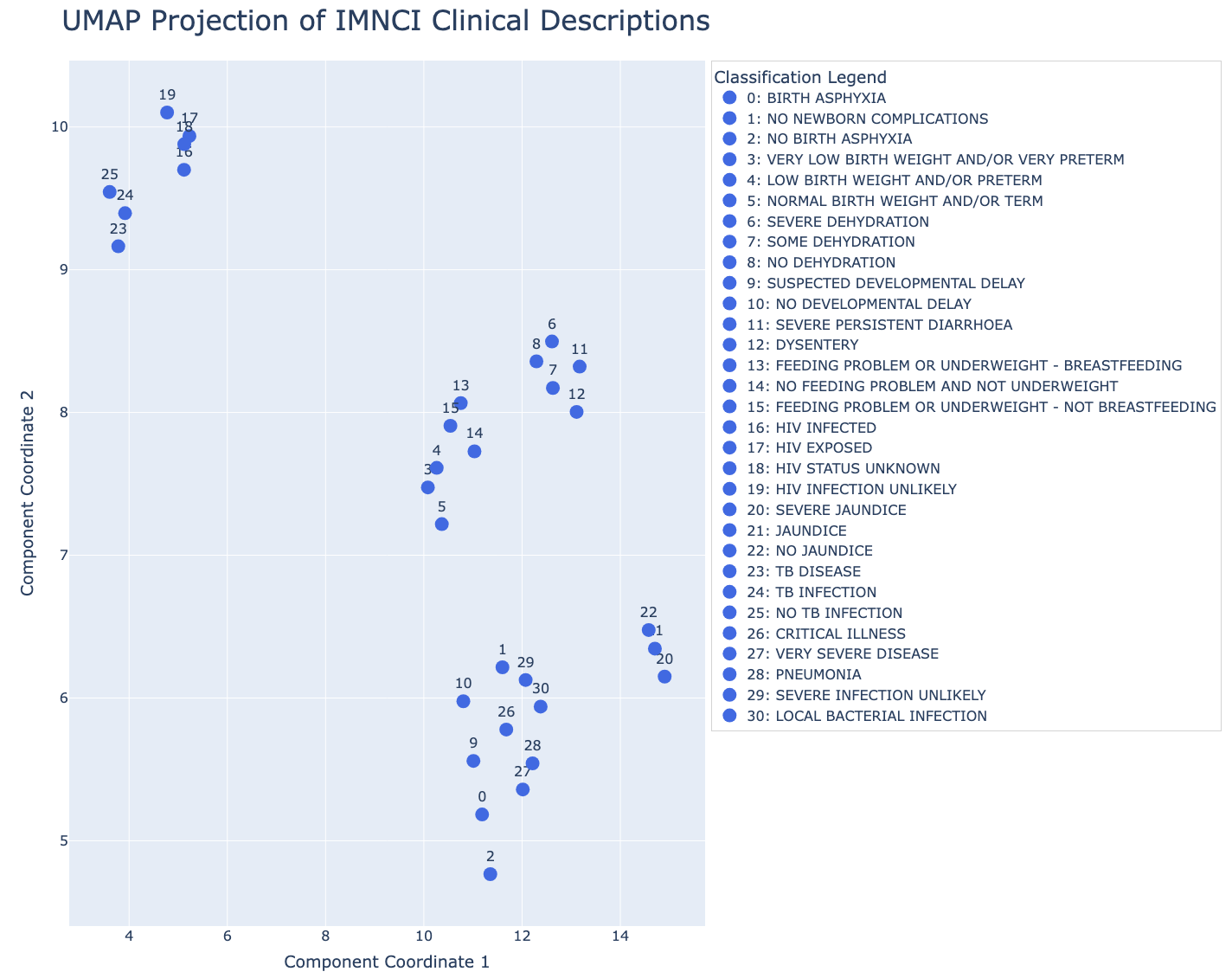
Prototype (LLR) Space

Prototype vectors spread widely across the diagnostic space. Each point reflects a condition’s weighted feature profile. Here, "16: NO JAUNDICE" and "23: SEVERE JAUNDICE" are clearly separated (despite using related clinical terminology) because they rely on different underlying features.

Are Prototype Vectors Useful For Semantic Search?

Not directly. A prototype vector isn’t a sentence or label. Rather, it’s a coordinate-weighted map of feature importance. If you feed a natural language query like “bloody stool diseases” into prototype space, you'll get meaningless results. That’s because the axes aren’t words—they’re LLR weights for features like “Yellow palms” or “Fast breathing.”

What prototype vectors are good for is clinical pattern matching. For example:

Query	Best Vector Space
“Which conditions mention ‘shortness of breath’ or look like pneumonia?”	Text embedding space
“Which conditions share nearly the same LLR-weighted features as acute malnutrition?”	Prototype vector space

When to Use Prototype Vectors

Here’s where prototype vectors are most useful:

1. Pattern similarity Identify conditions that share similar diagnostic signatures—ideal for exploring differential diagnoses or uncovering syndromic clusters.

2. Patient-to-condition scoring Quickly compute dot products between a sparse patient vector and all prototypes to get ranked condition scores.

3. Unsupervised clustering Use K-means or HDBSCAN on prototype vectors to discover latent families of conditions, based on shared diagnostic patterns instead of label semantics.

4. Explainability Each prototype is a transparent ranked list of LLR-weighted features. You can easily surface these in UI: “This condition is likely because of A, B, and C.”

Bridging Language and Evidence

If you want to accept natural language queries but return results based on diagnostic feature similarity, then you can:

1. Use an LLM or text-to-feature model to extract clinical signs

2. Map extracted phrases to known atomic features (e.g., via a lookup table or fuzzy matcher)

3. Construct a temporary sparse patient vector using those signs

4. Score similarity between the temporary patient vector and each prototype using dot product or cosine similarity

5. Return the top-ranked conditions

This gives you the best of both worlds:

• Natural language input
• Feature-based, explainable, evidence-grounded results

Key Takeaways

Use text embeddings for:

• Semantic search
• Documentation retrieval
• User-facing language interfaces

Use prototype vectors for:

• Condition risk scoring
• Feature-based search
• Clustering
• Explanation

From Prototype Vectors to Scoring Patients

Prototype vectors reflect how clinicians think: by weighing the presence (or absence) of concrete features to arrive at a diagnosis.

In the next section, we’ll show how to apply them to real patient data and turn these patient "fingerprints" into patient scores.

---

Scoring Patients: Clinical Evidence vs. Semantic Similarity

Now that we’ve built diagnostic fingerprints using LLRs, we can apply them to real patient cases—scoring how well each classification matches a patient’s observed features.

This allows us to move from clinical presentation to ranked diagnostic evidence.

Step 1: Convert Observations to Feature Vectors

Each synthetic patient case includes a list of clinical observations (e.g., “Low body temperature”, “Palms and/or soles yellow”). These are mapped to atomic features using the same lookup table we used to build prototypes.

The result is a sparse binary vector:

{
  "Yellow palms": 1,
  "Temperature: < 35.5°C": 1,
  ...
}

This vector represents the patient’s current clinical presentation.

Real-World Setting

In real-world deployment, these features would be extracted from free-text notes using standard NLP techniques or LLMs.

Step 2: Compute Evidence Scores

To score a patient against each classification, we compute the dot product between the patient’s feature vector and the prototype vector for that classification:

\[ \text{score}_{p,c} = \sum_{f \in F_p \cap F_c} w_{f,c} \]

Where:

• \(p\): the patient
• \(c\): a candidate classification
• \(F_p\): set of features present in patient \(p\)
• \(F_c\): set of features in the prototype vector for classification \(c\)
• \(w_{f,c}\): the LLR weight of feature \(f\) for classification \(c\)

In plain terms: sum the LLRs of all features shared by the patient and the prototype. Higher scores reflect stronger alignment.

What the Score Tells Us

• Positive scores = evidence supporting the diagnosis
• Near-zero or negative scores = little or no evidence

Because this scoring is additive and sparse, it’s:

• Efficient (no model inference required)
• Interpretable (each score = sum of traceable feature contributions)
• Flexible (handles partial matches well)

Example: LLR-Based Scoring Output

Below is the scoring output for a synthetic patient with low birth weight and uncertain HIV status:

{
  "Infant presented, mother confirmed HIV positive... baby is taking breast milk. Weight measured at 1900 grams. Definite low birth wt. Regarding baby's HIV status, the DNA PCR... uh, status unknown right now, maybe test not back yet? Need to confirm this. Baby seems small but... active.": {
    "HIV EXPOSED": 18.56384844577922,
    "LOW BIRTH WEIGHT AND/OR PRETERM": 11.192647708922227,
    "HIV INFECTION UNLIKELY": 2.4237972072938314,
    "NO TB INFECTION": 1.2408309180076675,
    "HIV INFECTED": 0.0,
    "NORMAL BIRTH WEIGHT AND/OR TERM": -0.6398399034175937,
    "HIV STATUS UNKNOWN": -1.5034183194330342,
    "NO BIRTH ASPHYXIA": -2.8842680613760097,
    "SEVERE INFECTION UNLIKELY": -3.081817340612081,
    "SEVERE PERSISTENT DIARRHOEA": -3.081817340612081,
    "TB INFECTION": -3.4552498829771383,
    "NO DEHYDRATION": -4.284004173563234,
    "NO JAUNDICE": -4.581105224483713,
    "TB DISEASE": -4.581105224483713,
    "SUSPECTED DEVELOPMENTAL DELAY": -5.502871189280269,
    "VERY LOW BIRTH WEIGHT AND/OR VERY PRETERM": -5.621976531201259,
    "NO FEEDING PROBLEM AND NOT UNDERWEIGHT": -6.179251620739574,
    "PNEUMONIA": -6.486742178054019,
    "NO DEVELOPMENTAL DELAY": -7.874434818099221,
    "DYSENTERY": -8.584653002684437,
    "NO NEWBORN COMPLICATIONS": -9.768618610148906,
    "LOCAL BACTERIAL INFECTION": -10.127362535042389,
    "FEEDING PROBLEM OR UNDERWEIGHT - NOT BREASTFEEDING": -11.741074723950456,
    "SEVERE DEHYDRATION": -12.682999177039619,
    "CRITICAL ILLNESS": -13.850710866467722,
    "FEEDING PROBLEM OR UNDERWEIGHT - BREASTFEEDING": -13.850710866467722,
    "SOME DEHYDRATION": -14.580684182715856,
    "SEVERE JAUNDICE": -14.711906429369382,
    "JAUNDICE": -16.007995284983828,
    "BIRTH ASPHYXIA": -17.391197577631043,
    "VERY SEVERE DISEASE": -18.16792519100755
  }
}

Top-scoring classifications are well-aligned with observed features; negative scores indicate poor matches.

This scoring method mirrors how clinicians accumulate evidence during diagnosis:

“The infant is underweight, breastfed, and has delayed developmental signs. These are clear indicators of multiple overlapping conditions.”

Semantic Similarity vs. Evidence Matching

To contrast approaches, we compare:

• Text Embeddings (semantic match to the observation text)
• Prototype Vectors (feature-based LLR match)

In the following table, each row shows:

• A synthetic patient observation note
• The (unordered) ground-truth classifications
• The top 3 results retrieved using text embeddings (semantic similarity via cosine score)
• The top 3 results retrieved using prototype vectors (evidence score via LLR dot product)

(Synthetic) Observation Note	Ground Truth Classifications (Unordered)	Top 3 (Text Embeddings with Similarity Score)	Top 3 (Prototype Vectors with LLR Score)
"Infant, mum thinks about 7 weeks old maybe... brought in because she says \"He only feeds a few times a day, maybe 6?\". On exam, baby seems... small? Can't weigh him now, scale is being used elsewhere. Attachment to breast looks a bit shallow, maybe that's why... hmm. Also, noticed he doesn't really follow my penlight much, and didn't jump when I clapped. Just sort of... blinked. Is he meeting his milestones? Need to check properly, but seems a bit delayed perhaps."	1. FEEDING PROBLEM OR UNDERWEIGHT - BREASTFEEDING 2. SUSPECTED DEVELOPMENTAL DELAY	1. FEEDING PROBLEM OR UNDERWEIGHT - BREASTFEEDING (0.56) 2. SUSPECTED DEVELOPMENTAL DELAY (0.55) 3. NO FEEDING PROBLEM AND NOT UNDERWEIGHT (0.54)	1. FEEDING PROBLEM OR UNDERWEIGHT - BREASTFEEDING (15.39) 2. SUSPECTED DEVELOPMENTAL DELAY (6.04) 3. NO TB INFECTION (1.25)
"infant breathing slow... <30? poor effort since birth. mother hiv status unknown, no test avail."	1. BIRTH ASPHYXIA 2. HIV STATUS UNKNOWN	1. HIV STATUS UNKNOWN (0.57) 2. HIV INFECTION UNLIKELY (0.55) 3. HIV EXPOSED (0.55)	1. HIV STATUS UNKNOWN (7.60) 2. BIRTH ASPHYXIA (6.87) 3. NO TB INFECTION(1.47)
"Infant presents with marked lethargy, responding only minimally when stimulated. Obvious sunken eyes noted on examination. Skin turgor appears significantly reduced; pinch retracts very slowly, though full assessment is challenging given the infant's condition. Overall impression is one of severe dehydration requirng urgent attention."	1. SEVERE DEHYDRATION	1. SEVERE DEHYDRATION (0.77) 2. SOME DEHYDRATION (0.70) 3. NO DEHYDRATION (0.68)	1. SEVERE DEHYDRATION (11.97) 2. SEVERE PERSISTENT DIARRHOEA (2.60) 3. DYSENTERY (0.67)
"6wk old infant here w/ mom. She states "watery stools for maybe 2 wks". looks tired. eyes sunken ++. skin pinch slowish return. fussy when examind. seems irritable. otherwise moving ok for now. no temp yet - machine in use. assess dehydration further."	1. SEVERE PERSISTENT DIARRHOEA 2. SOME DEHYDRATION	1. SOME DEHYDRATION (0.64) 2. SEVERE DEHYDRATION (0.61) 3. NO DEHYDRATION (0.59)	1. SEVERE PERSISTENT DIARRHOEA (15.16) 2. SOME DEHYDRATION (13.34) 3. DYSENTERY (8.58)
"vry small bb. looks premie maybe <32wk?. barely breathing, just gasps. mom says 'born too early'. no scale but looks v low wt prob <1.5kg. critical need help now."	1. BIRTH ASPHYXIA 2. VERY LOW BIRTH WEIGHT AND/OR VERY PRETERM	1. VERY LOW BIRTH WEIGHT AND/OR VERY PRETERM (0.55) 2. LOW BIRTH WEIGHT AND/OR PRETERM (0.52) 3. NORMAL BIRTH WEIGHT AND/OR TERM (0.47)	1. VERY LOW BIRTH WEIGHT AND/OR VERY PRETERM (12.85) 2. BIRTH ASPHYXIA (12.79) 3. NO TB INFECTION (2.03)

Text embeddings prioritize surface similarity and linguistic context. Prototype vectors, on the other hand, prioritize structured, feature-based evidence, leading to better clinical alignment, especially when phrasing is noisy or ambiguous.

Note how the cosine similarity scores in the text embedding column tend to cluster closely together, while the prototype LLR scores often show strong separation between the correct diagnosis and the rest. This separation reflects higher confidence and greater discriminative power, both of which are crucial for clinical decision-making.

Discriminative Power: Score Separation Matters

LLR-based scoring yields clear gaps between top and lower-ranked conditions. This enables:

• High-confidence triage
• Threshold-based alerts
• Explainable cutoffs for clinical action

In contrast, text similarity tends to return similar scores for many labels, even when the match is poor.

More separation = better triage, fewer false positives, and higher trust.

Interpretable Risk Banding with LLR Scores

Beyond ranking conditions, the additive nature of LLR-based scoring enables us to define risk bands. These are thresholds that convert evidence scores into interpretable clinical categories.

Let’s walk through a concrete example.

Suppose a patient presents with:

• Chest indrawing (LLR = 1.8)
• Respiratory rate ≥ 60 bpm (LLR = 0.9)
• Cough (LLR = 0.4)

Their total score for PNEUMONIA would be:

\[ \text{score}_{\text{PNEUMONIA}} = 1.8 + 0.9 + 0.4 = \mathbf{3.1} \]

This score alone is informative but becomes even more actionable when placed into a clinically meaningful band using simple, empirically derived thresholds:

Score Range	Risk Band
< 1.0	Low
1.0–2.5	Moderate
> 2.5	High

This banding provides intuitive stratification:

• Low Risk (< 1.0) Minimal evidence—likely not present, or ruled out by other features.

• Moderate Risk (1.0–2.5) Some evidence present—worth monitoring or gathering additional information.

• High Risk (> 2.5) Strong alignment with prototype—may justify diagnosis or intervention.

Visualizing Risk Scores

We can also visualize how a patient’s scores fall into risk bands across conditions:

Patient LLR scores mapped across different classifications. Prototype-based scoring reveals clear evidence stratification, making it ideal for thresholding, triage, and prioritization.

In our example, the PNEUMONIA score of 3.1 clearly falls in the High Risk band, indicating strong evidence and triggering diagnostic action.

Recap: Evidence-Based Scoring in Action

• Simplicity: No need for black-box thresholds or learned cutoffs. LLRs are additive and grounded in statistical reasoning.
• Interpretability: Each band maps directly to the number and quality of supporting features.
• Trust: Clinicians and users can trace how scores translate into risk assessments.

By moving from continuous scores to labeled bands, we bring LLR-based retrieval closer to real-world triage, prioritization, and explainable AI support.

In the next section, we’ll take it one step further and apply Bayes’ rule to convert these evidence scores into posterior probabilities.

---

Updating Beliefs with Bayesian Inference

So far, we’ve computed evidence scores that reflect how well each condition matches a patient’s observed features.

Now we take the final step: turning these raw scores into posterior probabilities using Bayes’ rule. This gives us a complete, probabilistic view of the patient’s likely diagnoses.

From LLR Scores to Probabilities

Each evidence score represents a sum of log-likelihood ratios (LLRs), which places it in log-odds space.

We can use this to compute the posterior odds of each diagnosis:

\[ \text{Posterior odds} = \text{Likelihood ratio} \times \text{Prior odds} \]

Then convert to a probability:

\[ P(c \mid f) = \frac{o(c \mid f)}{1 + o(c \mid f)} \]

Where:

• \(c\) = classification
• \(f\) = observed features
• \(o(c) = \frac{P(c)}{1 - P(c)}\): prior odds
• \(e^{\text{score}_{p,c}}\): likelihood ratio (from the LLR dot product)

Step-by-Step

1. Compute prior odds from historical classification frequencies
2. Exponentiate LLR score to get likelihood ratio
3. Multiply by prior odds to get posterior odds
4. Convert to probability

Example Calculation

Let’s say a patient has an LLR score of 4.2 for SEVERE JAUNDICE.

\[ \text{Likelihood ratio} = e^{4.2} \approx 66.7 \]

If the prior probability of SEVERE JAUNDICE is 0.08:

\[ \text{Prior odds} = \frac{0.08}{0.92} = 0.087 \]

\[ \text{Posterior odds} = 66.7 \times 0.087 \approx 5.80 \]

\[ P(c \mid f) = \frac{5.80}{1 + 5.80} \approx 0.85 \]

Interpretation: Even though the condition is rare (8% prior), the strong evidence raises the probability to 85%.

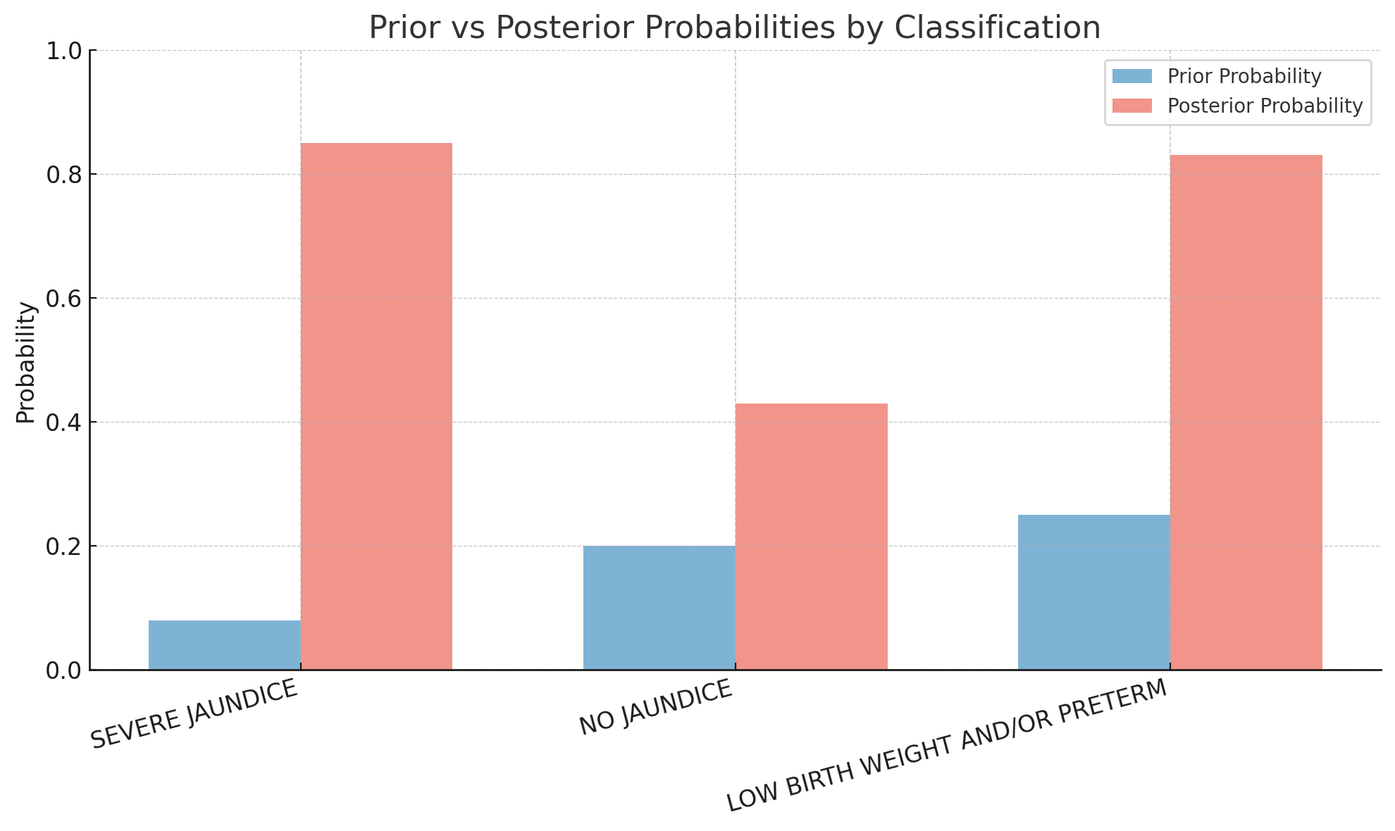
Bayesian Inference Table

The full Bayesian "inference table" for the patient might look like the following:

Bayesian Inference Table

Classification	Prior \( P(c) \)	Prior Odds \( o(c) \)	Score \( \text{score}_{p,c} \)	Likelihood Ratio \( e^{\text{score}_{p,c}} \)	Posterior Odds \( o(c \mid f) \)	Posterior \( P(c \mid f) \)
SEVERE JAUNDICE	0.08	0.087	4.2	66.69	5.80	0.85
NO JAUNDICE	0.20	0.25	1.1	3.00	0.75	0.43
LOW BIRTH WEIGHT AND/OR PRETERM	0.25	0.33	2.7	14.88	4.91	0.83

• SEVERE JAUNDICE and LOW BIRTH WEIGHT AND/OR PRETERM both end up with high posterior probabilities (~0.85 and ~0.83 respectively)
• This is consistent with the comorbid nature of the clinical presentation: both conditions are supported by the evidence
• NO JAUNDICE has a moderate prior but weak evidence, resulting in a relatively low posterior (~0.43)

Visualizing Prior vs. Posterior

Bayesian inference updates our beliefs by combining prior expectations with patient-specific evidence. Here, both `SEVERE JAUNDICE` and `LOW BIRTH WEIGHT` start with modest priors but rise dramatically after seeing strong supporting features. In contrast, `NO JAUNDICE` has a higher prior but receives little support from the patient’s presentation.

Example: Posterior Probabilities for a Patient

Let’s walk through the full posterior distribution for a synthetic patient:

Presentation: Lethargic infant, deeply sunken eyes, very slow skin pinch (>2 sec), reported bloody stools, poor feeding. Temperature not available.

{
    "SEVERE DEHYDRATION": 0.9671378689820405,
    "DYSENTERY": 0.9505448209234842,
    "VERY SEVERE DISEASE": 0.5025056758414613,
    "SEVERE PERSISTENT DIARRHOEA": 0.016517825862861567,
    "NO TB INFECTION": 0.00014444366452677872,
    "HIV INFECTED": 0.0001429592566118656,
    "HIV INFECTION UNLIKELY": 9.372854289907737e-05,
    "NORMAL BIRTH WEIGHT AND/OR TERM": 2.2356260007334426e-05,
    "HIV STATUS UNKNOWN": 9.474631018826278e-06,
    "NO BIRTH ASPHYXIA": 2.3970377466516665e-06,
    "SEVERE INFECTION UNLIKELY": 1.968886801059576e-06,
    "TB INFECTION": 1.3572133952041179e-06,
    "NO DEHYDRATION": 5.941789656207845e-07,
    "NO JAUNDICE": 4.4184363656549164e-07,
    "TB DISEASE": 4.4184363656549164e-07,
    "SUSPECTED DEVELOPMENTAL DELAY": 1.76195589439738e-07,
    "VERY LOW BIRTH WEIGHT AND/OR VERY PRETERM": 1.564549851034484e-07,
    "NO FEEDING PROBLEM AND NOT UNDERWEIGHT": 8.972165484732269e-08,
    "PNEUMONIA": 6.601203525422842e-08,
    "SOME DEHYDRATION": 1.896520840025167e-08,
    "NO DEVELOPMENTAL DELAY": 1.6518601246793633e-08,
    "NO NEWBORN COMPLICATIONS": 2.490764960428268e-09,
    "LOCAL BACTERIAL INFECTION": 1.740523814557602e-09,
    "LOW BIRTH WEIGHT AND/OR PRETERM": 1.6568266793199565e-09,
    "FEEDING PROBLEM OR UNDERWEIGHT - NOT BREASTFEEDING": 3.4705186895833757e-10,
    "HIV EXPOSED": 5.896893351131646e-11,
    "CRITICAL ILLNESS": 4.213652436632545e-11,
    "FEEDING PROBLEM OR UNDERWEIGHT - BREASTFEEDING": 4.213652436632545e-11,
    "SEVERE JAUNDICE": 1.7814662625972412e-11,
    "JAUNDICE": 4.875722983354526e-12,
    "BIRTH ASPHYXIA": 1.2229758833914898e-12
}

The ground truth classifications for this patient are:

• DYSENTERY
• SEVERE DEHYDRATION
• VERY SEVERE DISEASE

How This Compares

A standard vector database (semantic retrieval) returns:

• SEVERE DEHYDRATION
• SOME DEHYDRATION
• CRITICAL ILLNESS
• DYSENTERY
• VERY SEVERE DISEASE
• SEVERE PERSISTENT DIARRHOEA

While reasonable, this approach doesn’t offer confidence scores or distinguish sharply between likely and unlikely conditions.

What the Bayesian Engine Does Better

• High certainty for the key diagnoses:
  • SEVERE DEHYDRATION: 96.7%
  • DYSENTERY: 95.1%
• Moderate confidence for VERY SEVERE DISEASE: 50.3%
• All other conditions() are appropriately downweighted (most <0.001%)

This shows how Bayesian inference not only ranks conditions but also quantifies how likely each diagnosis is, accounting for comorbid conditions and overlapping features.

From Scores to Belief-Driven Triage

Bayesian inference lets us:

• Combine evidence and prevalence
• Support co-morbid diagnoses (multiple high posteriors)
• Calibrate scores into actionable probabilities

By combining prior prevalence and real-time evidence, the system provides interpretable, ranked probabilities, which are all critical for triage, risk stratification, and clinical support.

Real-World Uses

• Thresholding: Only show conditions with \( P > 0.25 \)
• Alerting: Highlight rare-but-likely diagnoses
• Clinical UI: Explain why each diagnosis is probable based on patient features

Closing the Loop

This step transforms our engine from a matching system to a true reasoning assistant. One that:

• Starts with structured features
• Scores evidence statistically
• Updates beliefs probabilistically
• Produces explainable, actionable output

In clinical settings, this kind of calibrated probability supports triage, differential diagnosis, and shared decision-making, especially in low-resource or high-stakes environments.

---

Bonus: Computing Log-Likelihood Ratios for Absent Features

So far, we’ve focused on the presence of features such as chest indrawing, yellow eyes, and rapid breathing as evidence for or against a diagnosis.

But in clinical reasoning, the absence of a finding can be just as telling:

• No chest indrawing? Pneumonia may be less likely.
• No blood in stool? Dysentery is less probable.

To capture this, we extend our LLR framework to include absent features. Absent features quantify how the lack of a finding shifts diagnostic belief.

How It Works

Let \(\neg f\) represent the absence of a feature \(f\). Then:

\[ \text{LLR}_{\neg f \rightarrow c} = \log \left( \frac{P(\neg f \mid c)}{P(\neg f \mid \neg c)} \right) \]

Where:

• \(P(\neg f \mid c)\): probability the feature is absent when the diagnosis is present
• \(P(\neg f \mid \neg c)\): probability the feature is absent when the diagnosis is absent

Example A: No Chest Indrawing → Pneumonia

	Pneumonia	Not Pneumonia
Absent	680	3820
Present	320	180

\[ \text{LLR}_{\neg f \rightarrow \text{PNEUMONIA}} = \log \left( \frac{0.68}{0.955} \right) \approx -0.34 \]

Interpretation: Weakly argues against pneumonia.

Example B: No Blood in Stool → Dysentery

	Dysentery	Not Dysentery
Absent	90	4800
Present	10	100

\[ \text{LLR}_{\neg f \rightarrow \text{DYSENTERY}} = \log \left( \frac{0.90}{0.979} \right) \approx -0.08 \]

Interpretation: Absence mildly lowers suspicion, but doesn’t rule it out.

Implementation Detail

We treat absence like any other feature:

• "Yellow palms" → LLR for presence
• "[ABSENT] Yellow palms" → LLR for absence

This gives us two-way reasoning with support from both presence and absence of features.

Why Absent Features Are Useful

Including absent-feature LLRs allows the system to:

• Account for negative evidence
• Support more nuanced diagnostic updates
• Improve coverage in incomplete notes

Sometimes what isn't present is just as meaningful as what is.

Future Extensions

In future models, we could represent patients with both:

• 1 → feature present
• -1 → feature explicitly absent
• 0 → feature unknown or unmentioned

This ternary encoding would unlock richer inference and more human-like diagnostic reasoning.

Final Thought

Diagnosis is often a process of exclusion as much as inclusion.

By modeling absent features as part of our probabilistic engine, we make the system more aligned with clinical intuition and more capable of robust, real-world decision support.

---

We hope this deep dive into Bayesian pattern recognition helps illuminate how probabilistic reasoning can enhance diagnostic systems, particularly in complex, multi-label clinical contexts.

Thanks for reading! If you're working on interpretable AI, pediatric decision support, or graph-based healthcare tools, we'd love to hear from you!

⬅️ Previous: Simulating Real World Pediatric Encounters Using Large Language Models

➡️ Next up: Evaluating GraphRAG vs. RAG on Real-World Messages

References

1. Likelihood ratios in diagnostic testing

Comments